Paper example : Clustering of 10k PBMCs sequenced by 10X scRNA-seq
To run this notebook you will need to download the data from Zenodo:
wget https://zenodo.org/records/10926960/files/10k_pbmc_gene.zip
unzip 10k_pbmc_gene.zip
Set the path to the data in settings/paths.py (rootFolder variable), and use the notebooks located in docs/examples/. Make sure to be in the repository root folder when launching notebooks, or use os.chdir() within the notebook. The notebook also requires the scran R dependency, but this can be bypassed using a different normalization approach.
First, load dependencies and setup the path to the dataset.
[16]:
import sys
sys.path.append("./")
import pandas as pd
import numpy as np
import os
import muffin
import scanpy as sc

dataset_path = "10k_pbmc_gene/"
You can set plot settings for muffin :
[17]:
try:
    os.mkdir("10k_pbmcs_results/")
except FileExistsError:
    pass
muffin.params["autosave_plots"] = "10k_pbmcs_results/"
muffin.params["figure_dpi"] = 96
muffin.params["autosave_format"] = ".pdf"
sc.set_figure_params(dpi=96, dpi_save=96, vector_friendly=True)
sc.set_figure_params(dpi=96, dpi_save=96, vector_friendly=True)
sc.settings.autosave = True
sc.settings.figdir = "10k_pbmcs_results/"
# Makes pdf font editable with pdf editors
import matplotlib as mpl
mpl.rcParams['pdf.fonttype'] = 42
We can load the dataset using scanpy functions, however muffin does not support sparse matrices :
[18]:
dataset = sc.read_10x_mtx(dataset_path + "filtered_feature_bc_matrix/")
dataset.X = dataset.X.astype(np.int32).toarray()
The dataset is in an anndata object, which allows for an easy annotation of the count matrix, and the storage of different count transforms. Results will be stored in this object.
[19]:
print(dataset)
AnnData object with n_obs × n_vars = 11996 × 36601
    var: 'gene_ids', 'feature_types'
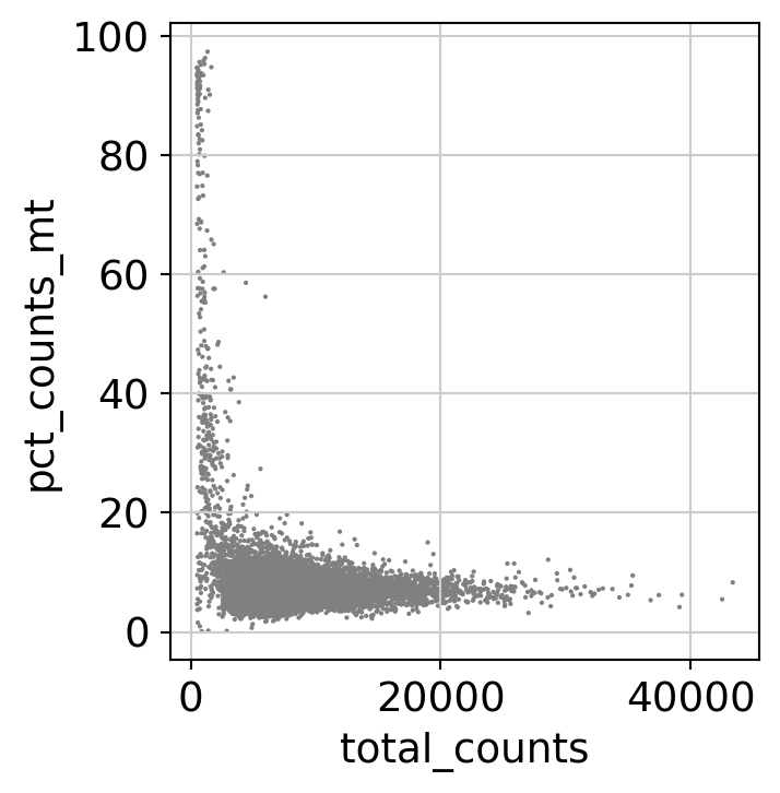
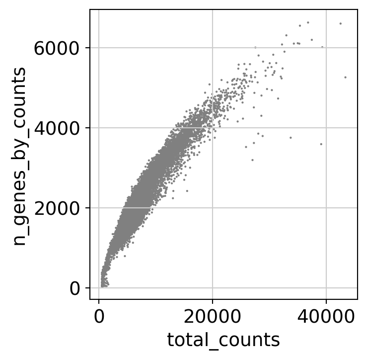
Here, we perform some standard QC (counts, percentage of mitochondrial RNA, number of detected genes…) on cells to remove low quality cells.
[20]:
dataset.var['mt'] = dataset.var_names.str.startswith('MT-')  # annotate the group of mitochondrial genes as 'mt'
sc.pp.calculate_qc_metrics(dataset, qc_vars=['mt'], percent_top=None, log1p=False, inplace=True)
sc.pl.scatter(dataset, x='total_counts', y='pct_counts_mt')
sc.pl.scatter(dataset, x='total_counts', y='n_genes_by_counts')
dataset = dataset[dataset.obs.pct_counts_mt < 15, :]
dataset = dataset[dataset.obs.n_genes_by_counts < 4000, :]
dataset = dataset[dataset.obs.n_genes_by_counts > 1000, :]
WARNING: saving figure to file 10k_pbmcs_results/scatter.pdf
WARNING: saving figure to file 10k_pbmcs_results/scatter.pdf
Here, we set up the design matrix of the linear model. If you do not want to regress any confounding factors leave it to a column array of ones as in the example. Note that it can have a tendency to “over-regress” and remove biological signal as it is a simple linear correction.
[21]:
design = np.ones((dataset.X.shape[0],1))
muffin.load.set_design_matrix(dataset, design)
Now, we are going to normalize library sizes using the scran approach, which is well suited to a large number of observations and small counts with many zeroes. We are also going to remove features with very low signal (note that this is mandatory to remove all zero counts).
[22]:
detectable = muffin.tools.trim_low_counts(dataset)
dataset = dataset[:, detectable]
muffin.tools.compute_size_factors(dataset, "scran")
[22]:
AnnData object with n_obs × n_vars = 10877 × 21890
    obs: 'n_genes_by_counts', 'total_counts', 'total_counts_mt', 'pct_counts_mt', 'size_factors'
    var: 'gene_ids', 'feature_types', 'mt', 'n_cells_by_counts', 'mean_counts', 'pct_dropout_by_counts', 'total_counts'
    obsm: 'design'
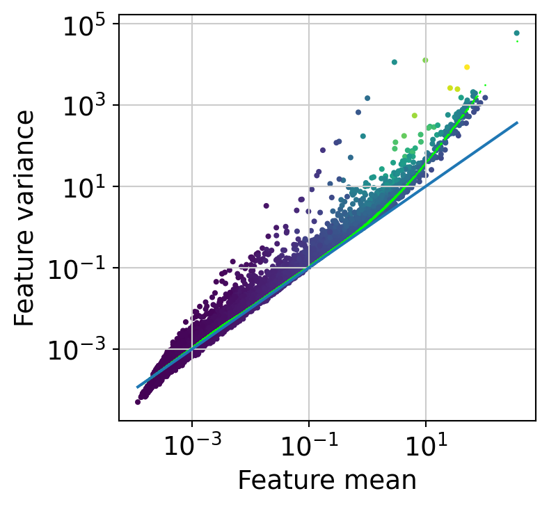
The next step is to fit the mean-variance relationship and compute residuals to the fitted Negative Binomial model.
[35]:
muffin.tools.compute_residuals(dataset, maxThreads=8)
[Parallel(n_jobs=8)]: Using backend LokyBackend with 8 concurrent workers.
[Parallel(n_jobs=8)]: Done 832 tasks      | elapsed:  2.3min
[Parallel(n_jobs=8)]: Done 2000 out of 2000 | elapsed:  3.4min finished
[Parallel(n_jobs=8)]: Using backend LokyBackend with 8 concurrent workers.
[Parallel(n_jobs=8)]: Done 16929 tasks      | elapsed:  3.2min
[Parallel(n_jobs=8)]: Done 21890 out of 21890 | elapsed:  3.6min finished
[35]:
AnnData object with n_obs × n_vars = 10877 × 21890
    obs: 'n_genes_by_counts', 'total_counts', 'total_counts_mt', 'pct_counts_mt', 'size_factors', 'leiden', 'Annotated clusters', 'SCTransform_clusters'
    var: 'gene_ids', 'feature_types', 'mt', 'n_cells_by_counts', 'mean_counts', 'pct_dropout_by_counts', 'total_counts', 'means', 'variances', 'reg_alpha'
    uns: 'pca', 'leiden_colors', 'rank_genes_groups', 'Annotated clusters_colors', 'dendrogram_Annotated clusters'
    obsm: 'design', 'X_pca', 'X_umap'
    varm: 'PCs'
    layers: 'residuals', 'scaled'
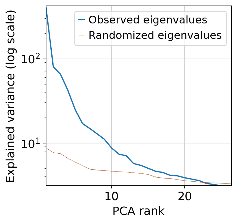
Next, we perform dimensionnality reduction with PCA (automatically finding the optimal dimensionnality) and UMAP.
[36]:
muffin.tools.compute_pa_pca(dataset, max_rank=50, plot=True)
muffin.tools.compute_umap(dataset)
[36]:
AnnData object with n_obs × n_vars = 10877 × 21890
    obs: 'n_genes_by_counts', 'total_counts', 'total_counts_mt', 'pct_counts_mt', 'size_factors', 'leiden', 'Annotated clusters', 'SCTransform_clusters'
    var: 'gene_ids', 'feature_types', 'mt', 'n_cells_by_counts', 'mean_counts', 'pct_dropout_by_counts', 'total_counts', 'means', 'variances', 'reg_alpha'
    uns: 'pca', 'leiden_colors', 'rank_genes_groups', 'Annotated clusters_colors', 'dendrogram_Annotated clusters'
    obsm: 'design', 'X_pca', 'X_umap'
    varm: 'PCs'
    layers: 'residuals', 'scaled'
Now, cluster the cells.
[37]:
muffin.tools.cluster_rows_leiden(dataset)
[37]:
AnnData object with n_obs × n_vars = 10877 × 21890
    obs: 'n_genes_by_counts', 'total_counts', 'total_counts_mt', 'pct_counts_mt', 'size_factors', 'leiden', 'Annotated clusters', 'SCTransform_clusters'
    var: 'gene_ids', 'feature_types', 'mt', 'n_cells_by_counts', 'mean_counts', 'pct_dropout_by_counts', 'total_counts', 'means', 'variances', 'reg_alpha'
    uns: 'pca', 'leiden_colors', 'rank_genes_groups', 'Annotated clusters_colors', 'dendrogram_Annotated clusters'
    obsm: 'design', 'X_pca', 'X_umap'
    varm: 'PCs'
    layers: 'residuals', 'scaled'
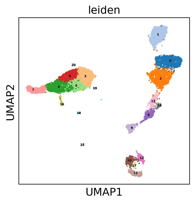
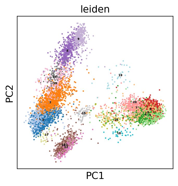
Display the results. Note that we can use scanpy functions here!
[38]:
# Append cell type info to the dataset
sc.pl.umap(dataset, color='leiden', legend_loc='on data',
                legend_fontsize=4, legend_fontoutline=0.1, s=15.0,
                palette='tab20')
sc.pl.pca(dataset, color='leiden', legend_loc='on data',
                legend_fontsize=4, legend_fontoutline=0.1, s=15.0,
                palette='tab20')
WARNING: saving figure to file 10k_pbmcs_results/umap.pdf
WARNING: saving figure to file 10k_pbmcs_results/pca.pdf
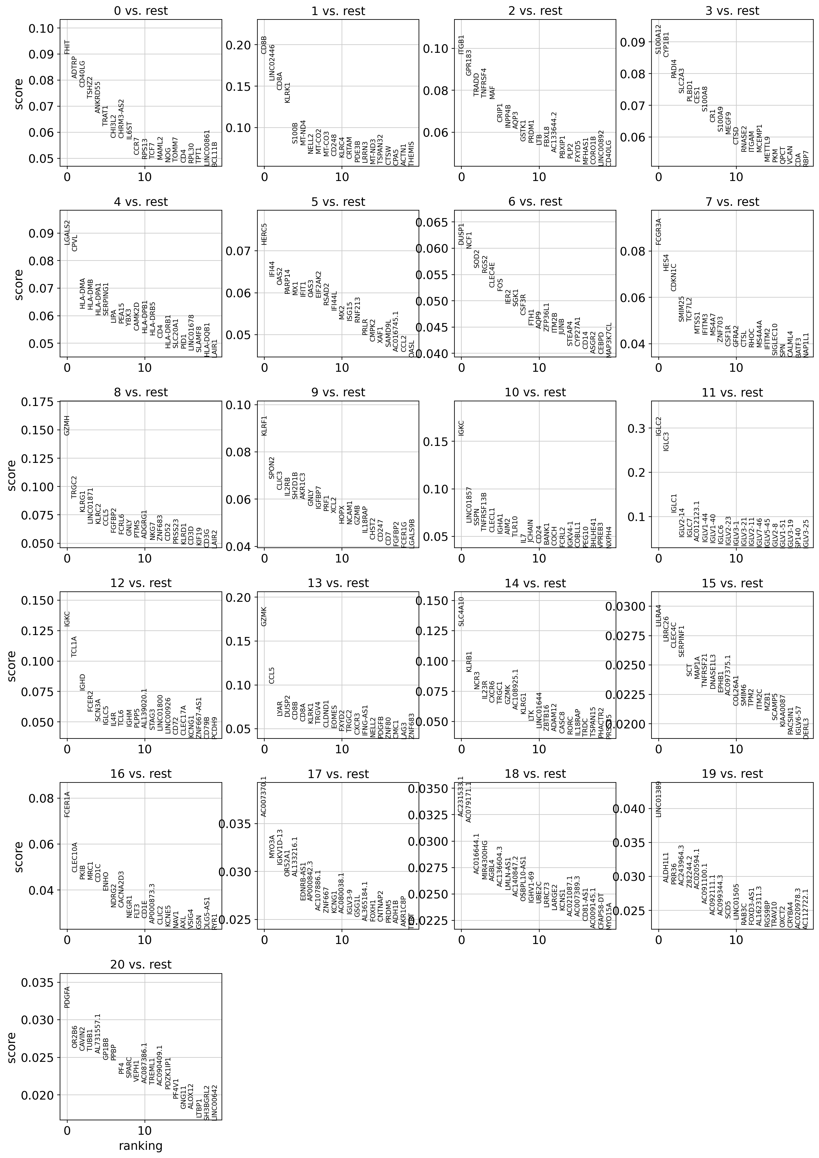
Let’s find markers using a logistic regression :
[61]:
from sklearn.preprocessing import StandardScaler
# It is strongly advised to standardize inputs for a better convergence of the solver (especially for large datasets).
dataset.layers["scaled"] = StandardScaler().fit_transform(dataset.layers["residuals"])
sc.tl.rank_genes_groups(dataset, 'leiden', use_raw=False, layer="scaled",
                        method='logreg', class_weight="balanced")
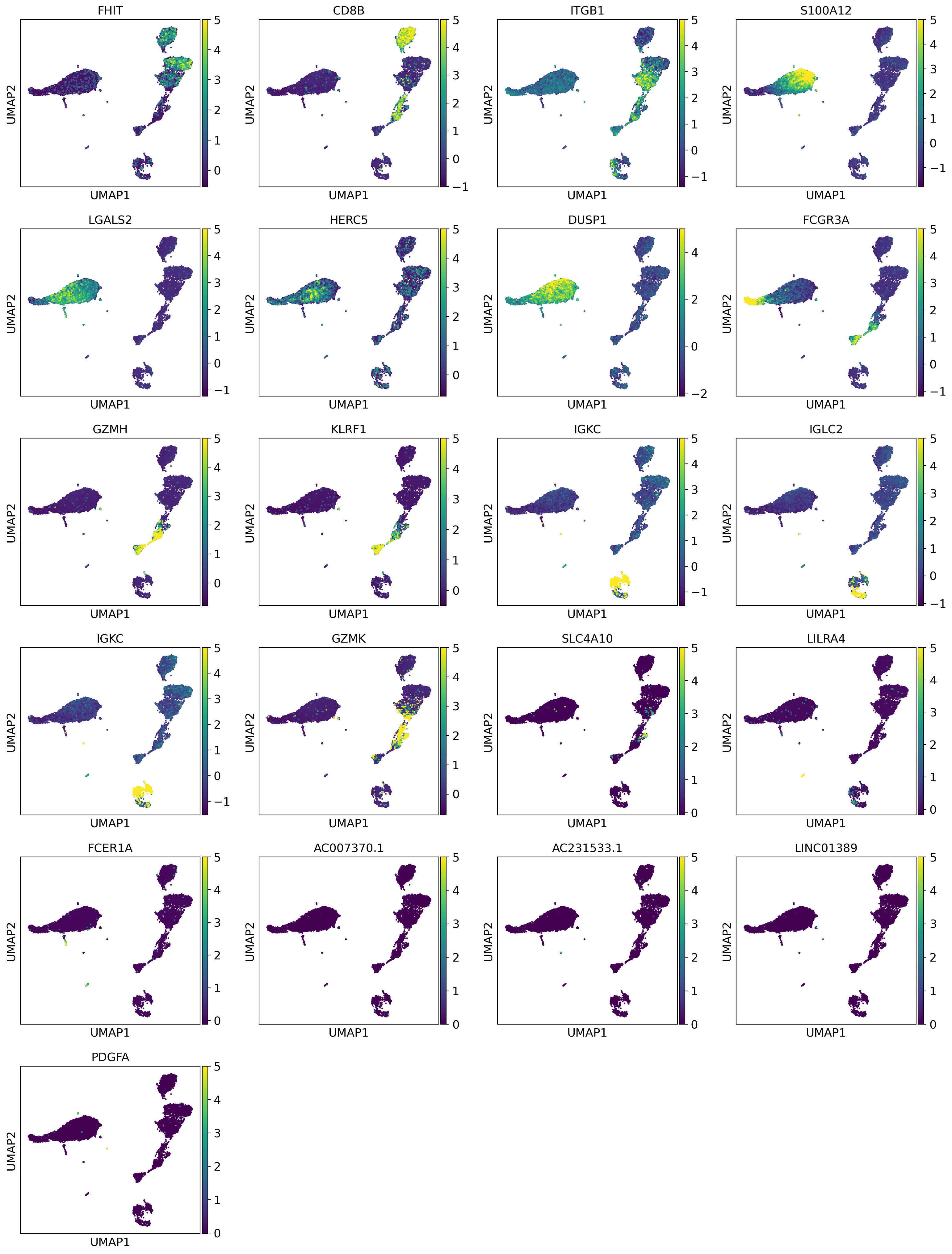
We can see some known markers of well-known cell types (CD8B for cluster 1 - CD8 T Cells, PPBP for cluster 20 - platelets):
[62]:
sc.pl.rank_genes_groups(dataset, sharey=False)
WARNING: saving figure to file 10k_pbmcs_results/rank_genes_groups_leiden.pdf
[63]:
bestmarkers = [dataset.uns["rank_genes_groups"]["names"][0][i] for i in range(len(dataset.uns["rank_genes_groups"]["names"][0]))]
sc.pl.umap(dataset, color=bestmarkers, vmax=5.0,
                legend_fontsize=4, legend_fontoutline=0.1, s=15.0,
                palette='tab20', layer="residuals", save=f"umap_markers.pdf")
WARNING: saving figure to file 10k_pbmcs_results/umapumap_markers.pdf
Let’s annotate cell types :
[64]:
cluster_names = {"0":"T-Cells CD4 Naive",
                 "1":"T-Cells CD8 Naive",
                 "2":"T-Cells CD4 Memory",
                 "3":"Monocytes S100A12+",
                 "4":"Monocytes LGALS2+",
                 "5":"Monocytes HERC2+",
                 "6":"Monocytes DUSP1+",
                 "7":"Monocytes FCGR3A+",
                 "8":"T-Cells CD8 GZMH+",
                 "9":"NK Cells",
                 "10":"B-Cells IGKC+",
                 "11":"B-Cells IGCL2+",
                 "12":"B-Cells IGKC+ TCL1A+",
                 "13":"T-Cells CD8 GZMK+",
                 "14":"T-Cells MAIT",
                 "15":"Plasmacytoid DC",
                 "16":"Myeloid DC",
                 "17":"B-Cells ?",
                 "18":"Monocytes ? 2",
                 "19":"Monocytes ?",
                 "20":"Platelets"}
dataset.obs["Annotated clusters"] = pd.Series(cluster_names)[dataset.obs["leiden"]].values
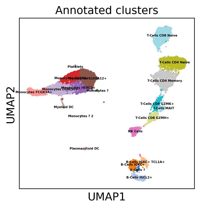
We can re-plot with annotated clusters
[65]:
sc.pl.umap(dataset, color="Annotated clusters",  s=15.0, legend_loc="on data", legend_fontsize=4,
                palette='tab20', layer="residuals", vmax=5, save=f"umap_annot.pdf")
WARNING: saving figure to file 10k_pbmcs_results/umapumap_annot.pdf
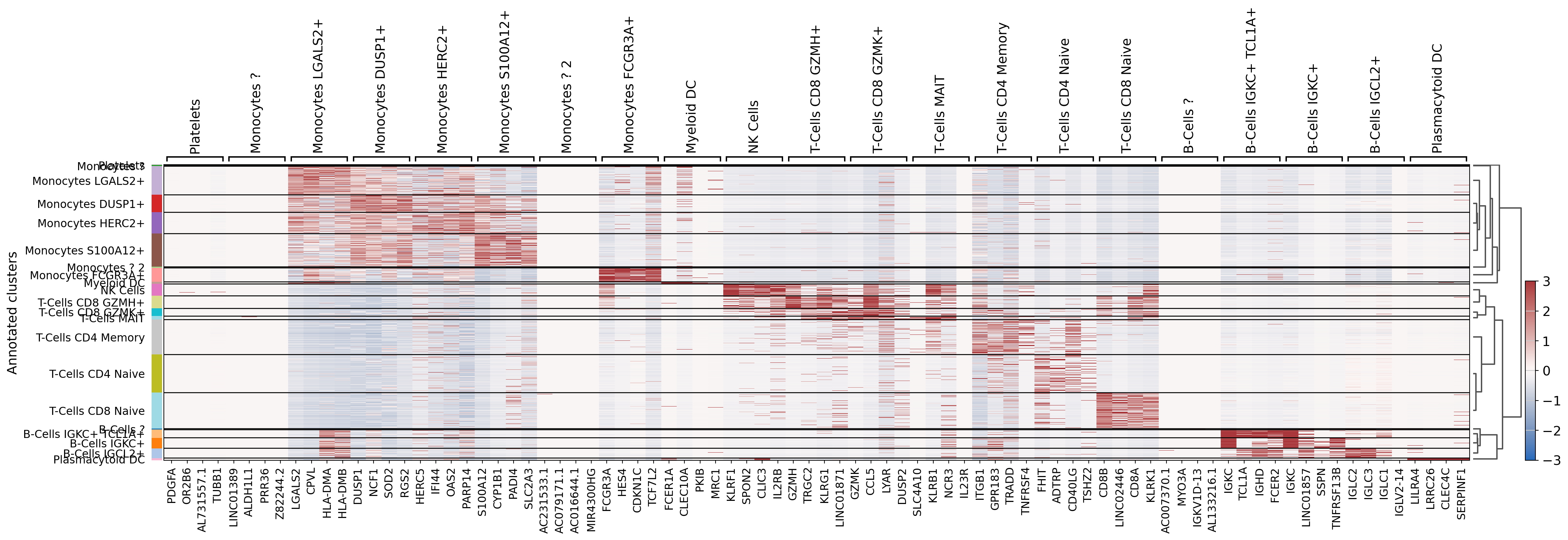
[66]:
# Ugly hack to solve an issue with scanpy logreg that does not output all fields
dataset.uns["rank_genes_groups"]["logfoldchanges"] = dataset.uns["rank_genes_groups"]["scores"]
dataset.uns["rank_genes_groups"]["pvals"] = dataset.uns["rank_genes_groups"]["scores"]
dataset.uns["rank_genes_groups"]["pvals_adj"] = dataset.uns["rank_genes_groups"]["scores"]
sc.tl.dendrogram(dataset, groupby="Annotated clusters", optimal_ordering=True, linkage_method="average")
sc.tl.rank_genes_groups(dataset, 'Annotated clusters', use_raw=False, layer="scaled",
                        method='logreg', class_weight="balanced")
sc.pl.rank_genes_groups_heatmap(dataset, layer="scaled", use_raw=False,
                                vmin=-3, vmax=3, cmap="vlag", show_gene_labels=True,
                                n_genes=4)
WARNING: saving figure to file 10k_pbmcs_results/heatmap.pdf
We can save our work to avoid recomputing everything. It can easily be re-loaded using : anndata.read_h5ad(path). We can also see that our dataset carries much more data than at the start.
[67]:
dataset.write("10k_pbmcs_results/dataset.h5ad")
print(dataset)
AnnData object with n_obs × n_vars = 10877 × 21890
    obs: 'n_genes_by_counts', 'total_counts', 'total_counts_mt', 'pct_counts_mt', 'size_factors', 'leiden', 'Annotated clusters', 'SCTransform_clusters'
    var: 'gene_ids', 'feature_types', 'mt', 'n_cells_by_counts', 'mean_counts', 'pct_dropout_by_counts', 'total_counts', 'means', 'variances', 'reg_alpha'
    uns: 'pca', 'leiden_colors', 'rank_genes_groups', 'Annotated clusters_colors', 'dendrogram_Annotated clusters'
    obsm: 'design', 'X_pca', 'X_umap'
    varm: 'PCs'
    layers: 'residuals', 'scaled'
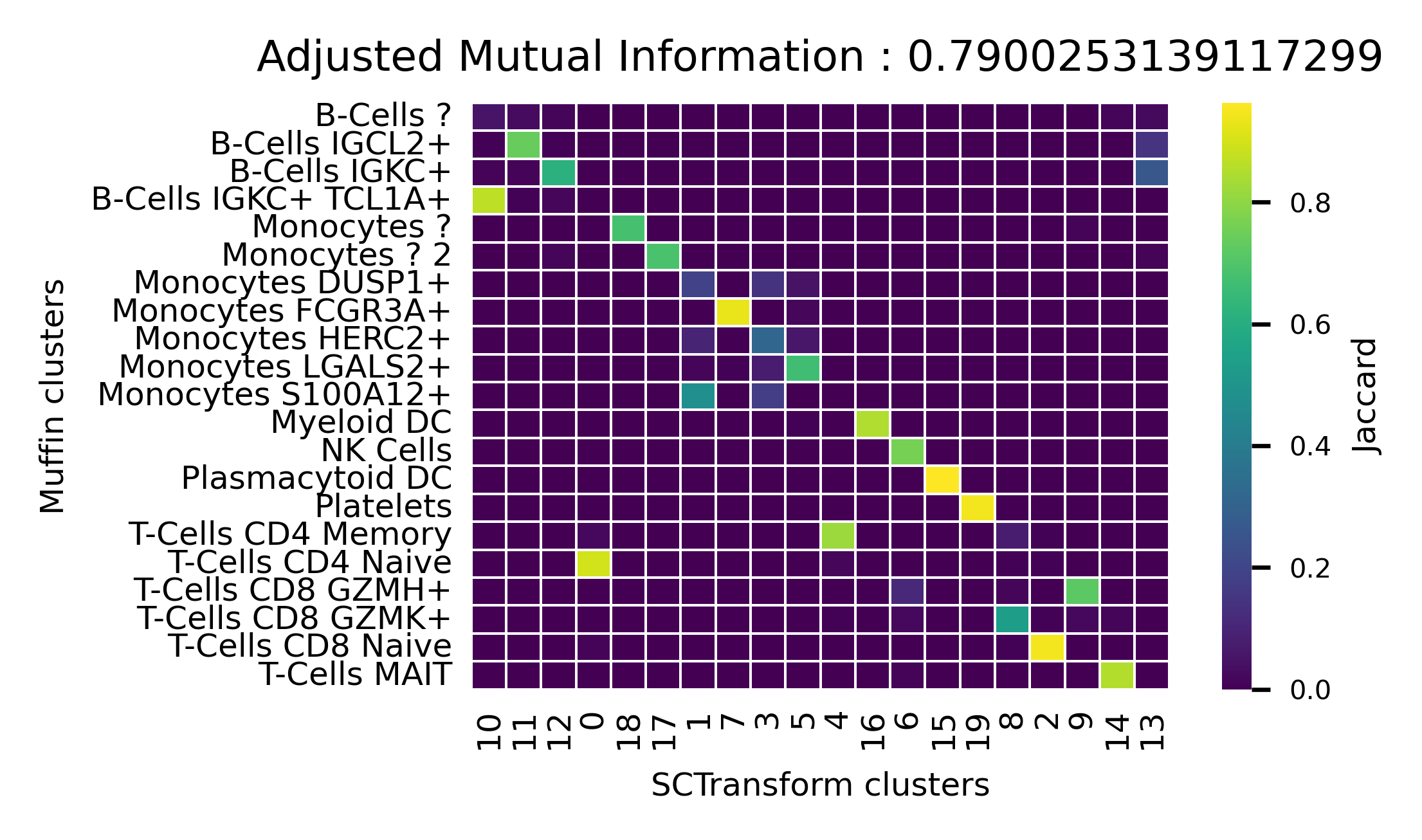
Figure 3C
[68]:
dataset.obs["SCTransform_clusters"] = pd.read_csv("benchmarks/scrnaseq/10k_pbmc_sct_clusters.csv", index_col=0, sep=",")["V1"]
from sklearn.metrics import adjusted_mutual_info_score
import matplotlib.pyplot as plt
import seaborn as sns
from scipy.spatial.distance import jaccard
# Build confusion matrix
unique_clust_muffin = np.unique(dataset.obs["Annotated clusters"])
unique_clust_sct = np.unique(dataset.obs["SCTransform_clusters"])
cm = pd.DataFrame(np.zeros((len(unique_clust_sct), len(unique_clust_muffin))),
                  columns=unique_clust_muffin, index=unique_clust_sct)
for i in unique_clust_muffin:
    for j in unique_clust_sct:
        cm.loc[j,i] = 1-jaccard(dataset.obs["Annotated clusters"].values==i,
                              dataset.obs["SCTransform_clusters"].values==j)
ami = adjusted_mutual_info_score(dataset.obs["Annotated clusters"].values, dataset.obs["SCTransform_clusters"].values)
# Greedily re-order cluster to match muffin clustering
orderlist = list(np.copy(unique_clust_sct))
reordered = []
for c in cm.columns:
    if len(orderlist) == 0:
        break
    reordered.append(cm.loc[orderlist,c].idxmax())
    orderlist.remove(cm.loc[orderlist,c].idxmax())
# Plot
plt.figure(dpi=300, figsize=(3.5,2))
ax=sns.heatmap(cm.loc[reordered].T, xticklabels=True, yticklabels=True,
            cbar_kws={'label': 'Jaccard'},cmap="viridis", linecolor="w", linewidths=0.25)
cbar = ax.collections[0].colorbar
cbar.ax.tick_params(labelsize=5)
ax.figure.axes[-1].yaxis.label.set_size(6)
plt.ylabel('Muffin clusters',fontsize=6)
plt.xlabel('SCTransform clusters',fontsize=6)
plt.yticks(fontsize=6)
plt.xticks(fontsize=6, rotation=90)
plt.grid(False)
plt.title(f"Adjusted Mutual Information : {ami}", fontsize=8)
plt.gca().set_aspect(1/1.25)
ax.tick_params(axis=u'both', which=u'both',length=0)
plt.savefig("10k_pbmcs_results/cluster_sim.pdf", bbox_inches="tight")
plt.show()