Paper example : H3K4Me3 occupancy in immune cells via ChIP-seq
To run this notebook you will need to download the data from Zenodo:
wget https://zenodo.org/records/10708208/files/immune_chip.zip
wget https://zenodo.org/records/10708208/files/GO_files.zip
wget https://zenodo.org/records/10708208/files/genome_annot.zip
unzip immune_chip.zip
unzip GO_files.zip
unzip genome_annot.zip
If you really wish to reproduce this notebook (WARNING : it will download around 100GB of data from ENCODE), you will need to run the the snakemake script “dl_data.smk” located in the immune_chip/ folder downloaded from the zenodo repository. The notebook also requires the rsubread, DESeq2 and apeglm R dependency.
First, load file metadata and dependencies. Note that rows in the metadata are already aligned to be from the same observation.
[5]:
import sys
sys.path.append("./")
sys.path.append("../..")
import pandas as pd
import numpy as np
import os
import muffin
import scanpy as sc

path_gencode, path_chromsizes, path_GOfile = "genome_annot/gencode.v38.annotation.gtf", "genome_annot/hg38.chrom.sizes.sorted",  "GO_files/hsapiens.GO:BP.name.gmt"
path_chip_data = "immune_chip/"
metadata_chip = pd.read_csv(path_chip_data+ "metadata_mod.tsv", sep="\t")
# List of paths to all files
bam_files = [path_chip_data + "chip/" + f + ".bam" for f in metadata_chip.loc[:, "ChIP"]]
input_files = [path_chip_data + "input/" + f + ".bam" for f in metadata_chip.loc[:, "Inputs"]]
peak_files = [path_chip_data + "peaks/" + f + ".bigBed" for f in metadata_chip.loc[:, "Peaks"]]
Now, we load the bed files for each experiment. Here they were in bigBed format so that takes a bit more code.
[6]:
import pyBigWig
def read_bigBed_encode(path):
    bb = pyBigWig.open(path)
    chroms = bb.chroms()
    entries_list = []
    for chrom, length in chroms.items():
        entries = bb.entries(chrom, 0, length)
        for entry in entries:
            entries_list.append({
                'chrom': chrom,
                'start': int(entry[0]),
                'end': int(entry[1]),
                'name': entry[2],
            })
    df = pd.DataFrame(entries_list)
    df[["name", "Score", "Strand", "FC", "Pval", "FDR", "Summit"]] = df["name"].str.split("\t", expand=True)
    df[["FC", "Pval", "FDR"]] = df[["FC", "Pval", "FDR"]].astype("float")
    df["Summit"] = df["Summit"].astype(int)
    return df
beds = [read_bigBed_encode(f) for f in peak_files]
# Not necessary
concat_bed = pd.concat(beds)
concat_bed.to_csv("h3k4me3_results/all_beds.bed",sep="\t",header=None,index=None)
Next, we will identify consensus peaks which merges similar peaks across experiments.
[7]:
chromSizes = pd.read_csv(path_chromsizes, sep="\t", header=None, index_col=0).iloc[:,0].to_dict()
consensus_peaks = muffin.merge_peaks(beds, chromSizes)
consensus_peaks.to_csv("h3k4me3_results/consensus_peaks.bed",sep="\t",header=None,index=None)
# Not needed anymore
del beds
Now that we have our genomic regions of interest, we can sample the sequencing signal in BAM files and generate the count matrix. Note that you can provide custom parameters for featureCounts here. Alternatively, instead of providing a dataframe for the query regions, you can provide a path to a bed or SAF file through the genomic_regions_path argument.
[ ]:
featureCountParams = {"nthreads":16, "allowMultiOverlap":True, "minOverlap":1,
                      "countMultiMappingReads":False}
dataset = muffin.load.dataset_from_bam(bam_files, genomic_regions=consensus_peaks,
                                       input_bam_paths=input_files,
                                       featureCounts_params=featureCountParams,chromsizes=chromSizes)
The dataset is in an anndata object, which allows for an easy annotation of the count matrix, and the storage of different count transforms.
[9]:
print(dataset)
AnnData object with n_obs × n_vars = 52 × 110245
    var: 'Chromosome', 'Start', 'End', 'Strand'
    uns: 'counts_random', 'tot_mapped_counts', 'input_random'
    layers: 'input'
You can set plot settings for muffin :
[10]:
try:
    os.mkdir("h3k4me3_results/")
except FileExistsError:
    pass
muffin.params["autosave_plots"] = "h3k4me3_results/"
muffin.params["figure_dpi"] = 200
muffin.params["autosave_format"] = ".pdf"
sc.set_figure_params(dpi=200, dpi_save=300)
sc.settings.autosave = True
sc.settings.figdir = "h3k4me3_results/"
# Makes pdf font editable with pdf editors
import matplotlib as mpl
mpl.rcParams['pdf.fonttype'] = 42
Here, we can re-name our features (columns of the count matrix) to the nearest gene’s name for convenience in downstream analyses. The dataset variable annotation has been automatically annotated with genomic locations in the previous step. Note that the gsea_obj object also provides functions for gene set enrichment of nearby genes.
[11]:
gsea_obj = muffin.great.pyGREAT(path_gencode, path_chromsizes, path_GOfile)
dataset.var_names = gsea_obj.label_by_nearest_gene(dataset.var[["Chromosome","Start","End"]]).astype(str)
Here, we set up the design matrix of the linear model. If you do not want to regress any confounding factors leave it to a column array of ones as in the example. Note that it can have a tendency to “over-regress” and remove biological signal as it is a simple linear correction.
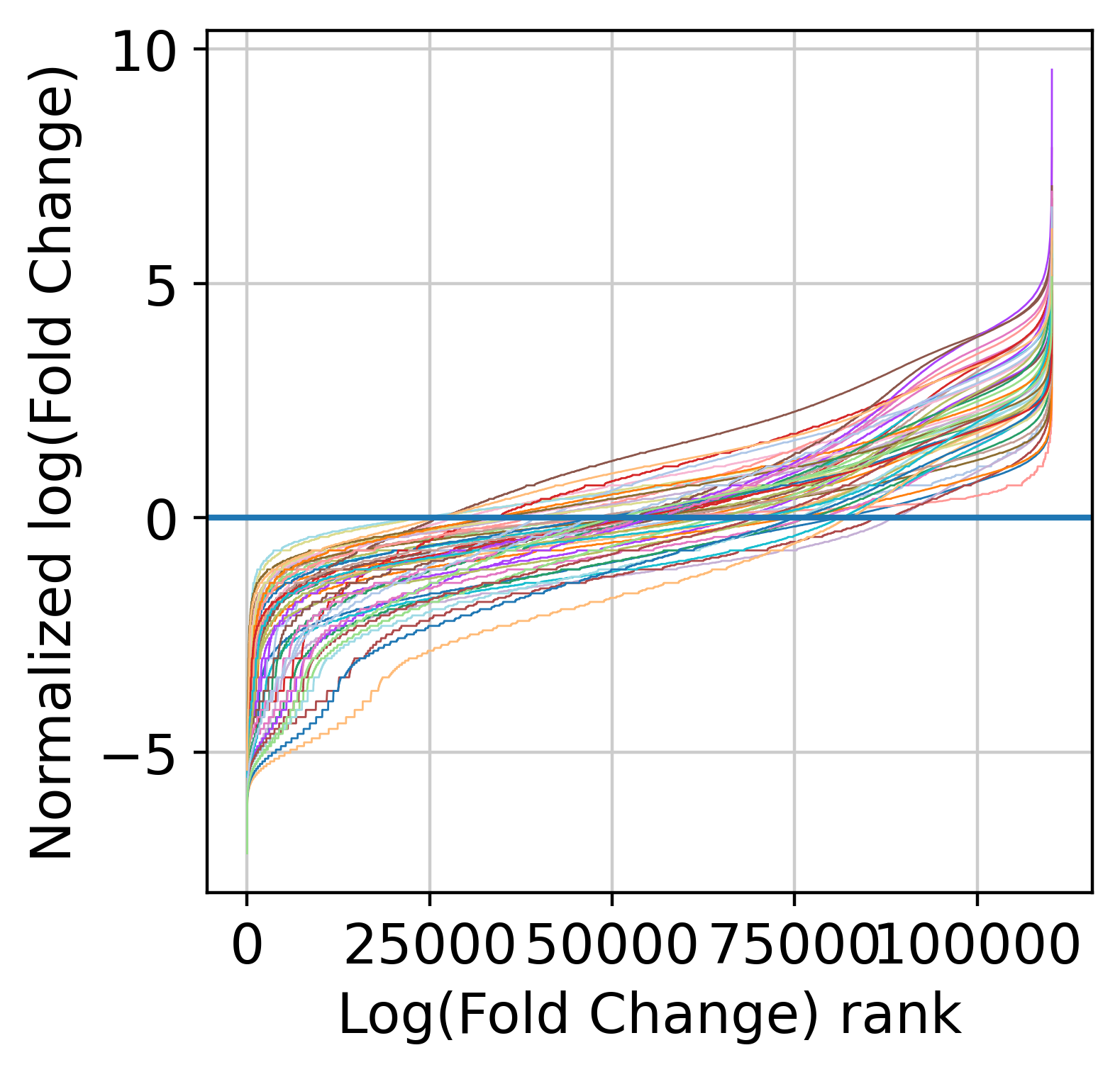
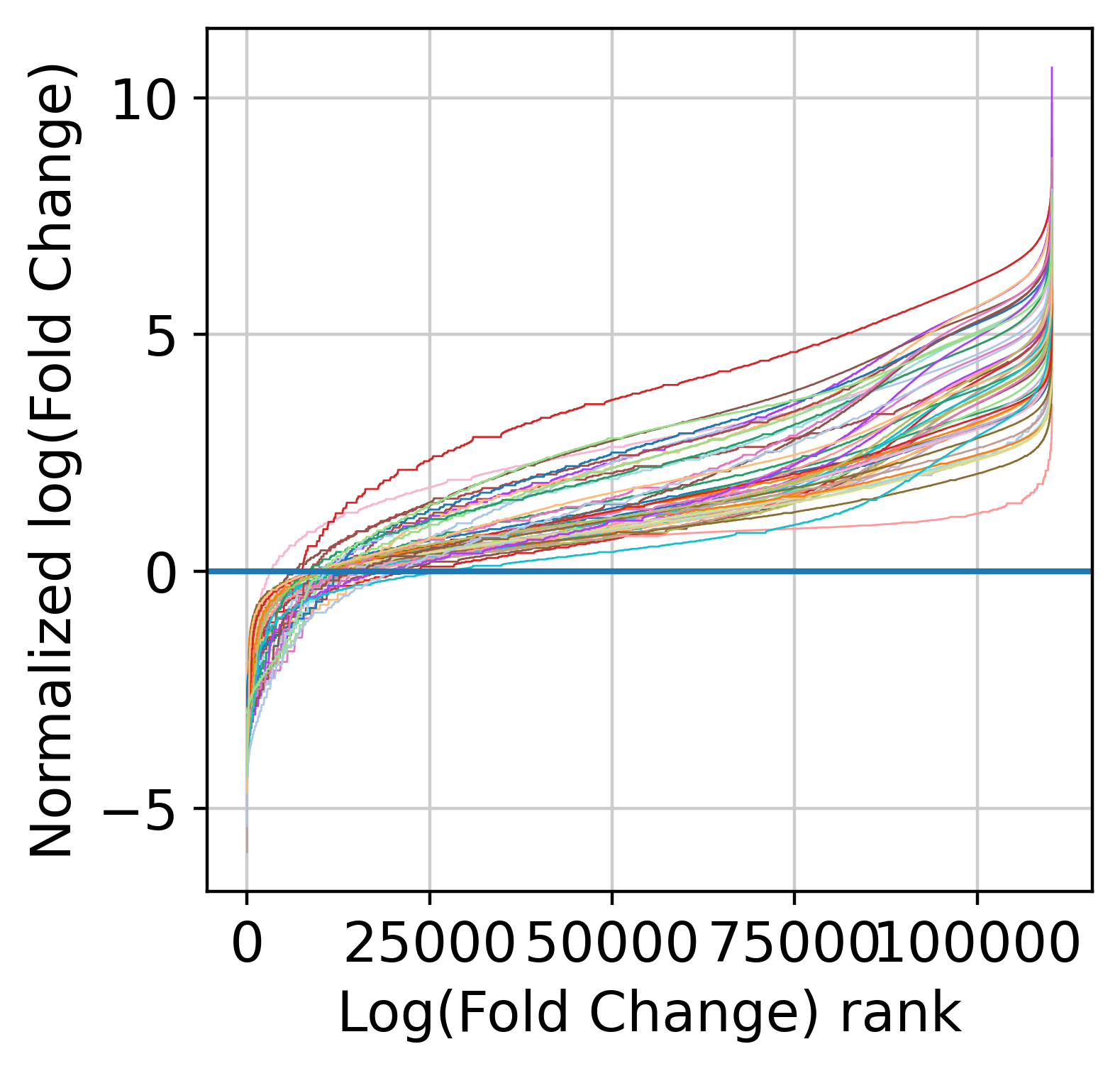
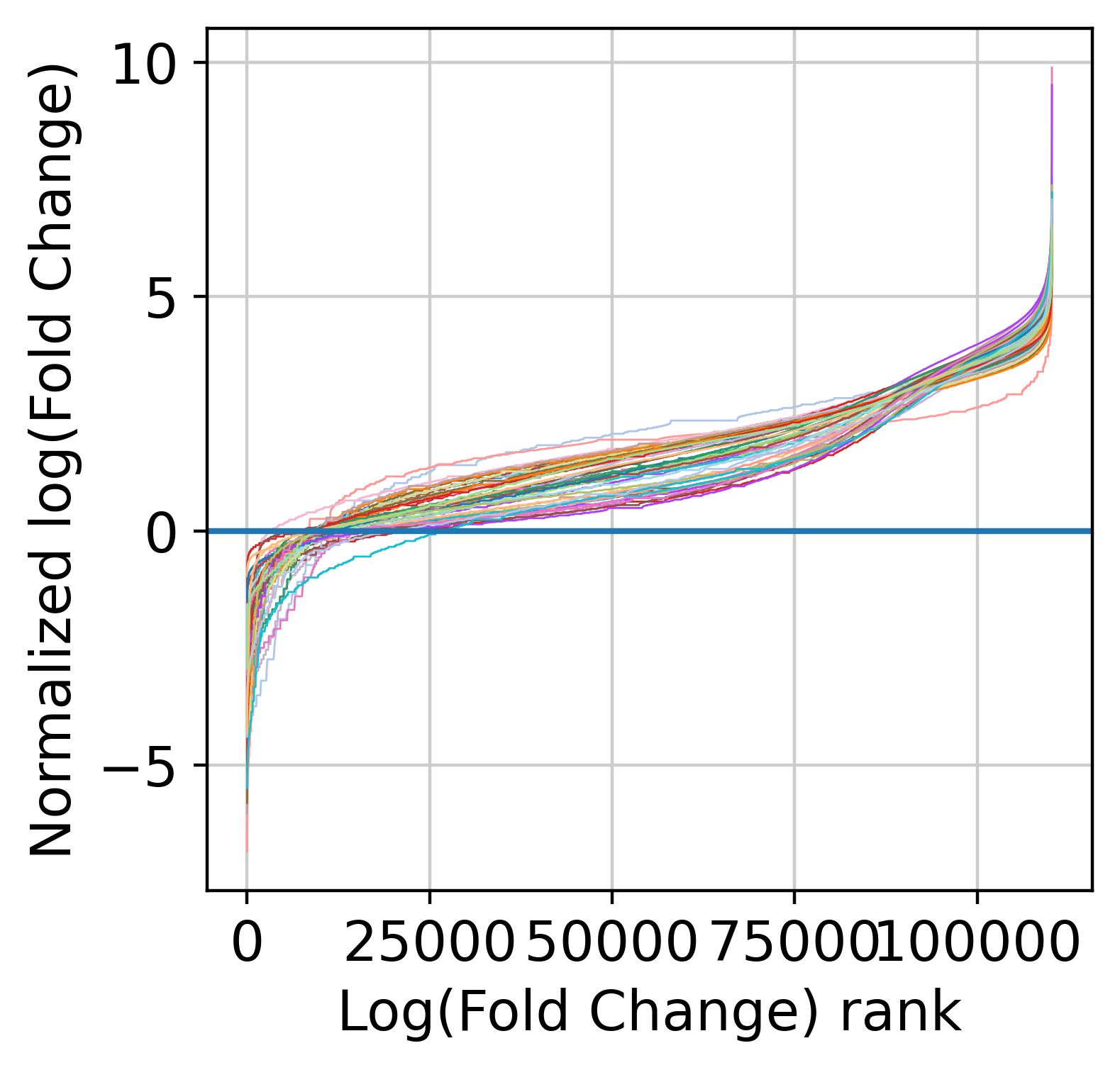
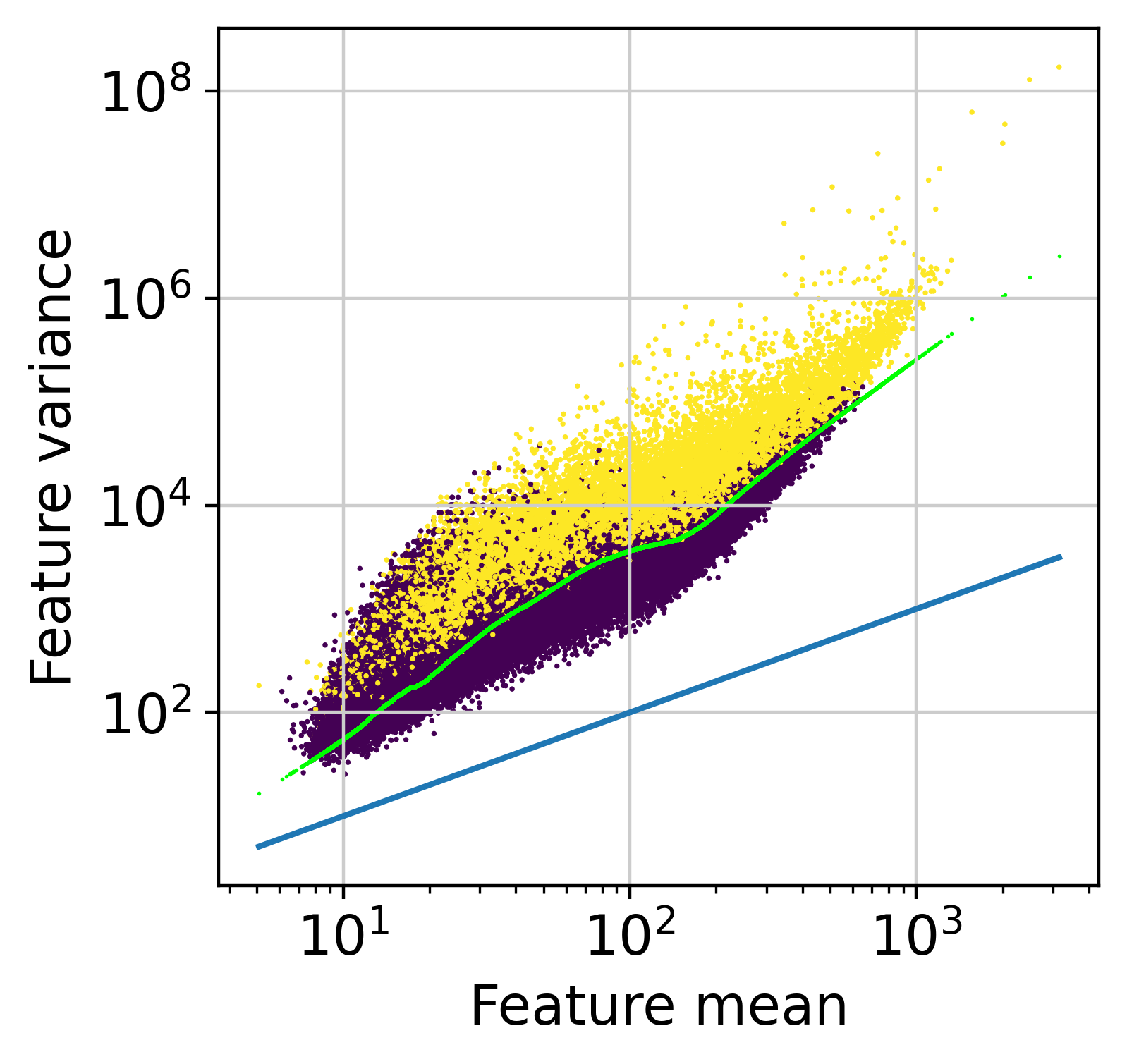
Now, we are count to normalize the input counts using our centering and scaling approach. Alternatively, you can use the rescale_input_quantile function. We are also going to remove features with very low signal (note that this step is mandatory to remove fully zero counts, which will cause numerical issues later on when fitting NB models).
[12]:
detectable = muffin.tools.trim_low_counts(dataset)
dataset = dataset[:, detectable]
muffin.tools.rescale_input_center_scale(dataset, plot=True)
design = np.concatenate([np.ones((len(dataset),1))], axis=1)
muffin.load.set_design_matrix(dataset, design)
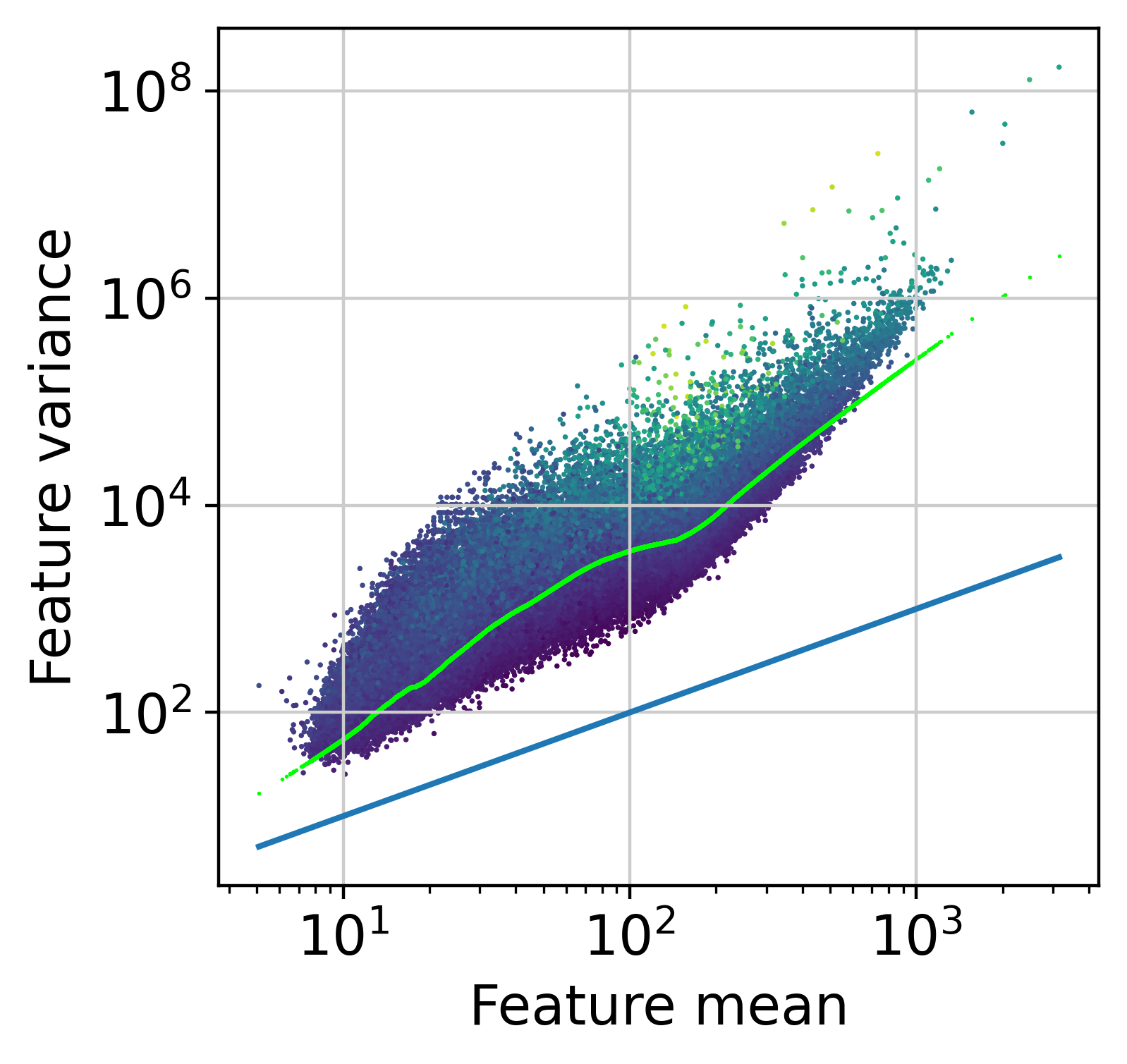
The next step is to fit the mean-variance relationship and the compute residuals to the fitted Negative Binomial model.
[13]:
muffin.tools.compute_residuals(dataset, residuals="quantile", maxThreads=16)
[Parallel(n_jobs=16)]: Using backend LokyBackend with 16 concurrent workers.
[Parallel(n_jobs=16)]: Done 358 tasks      | elapsed:   52.1s
[Parallel(n_jobs=16)]: Done 2000 out of 2000 | elapsed:  1.0min finished
[Parallel(n_jobs=16)]: Using backend LokyBackend with 16 concurrent workers.
[Parallel(n_jobs=16)]: Done 9248 tasks      | elapsed:  1.4min
[Parallel(n_jobs=16)]: Done 86048 tasks      | elapsed:  3.4min
[Parallel(n_jobs=16)]: Done 110245 out of 110245 | elapsed:  3.7min finished
[13]:
AnnData object with n_obs × n_vars = 52 × 110245
    obs: 'size_factors', 'size_factors_input', 'centered_lfc', 'pi0'
    var: 'Chromosome', 'Start', 'End', 'Strand', 'means', 'variances', 'reg_alpha'
    uns: 'counts_random', 'tot_mapped_counts', 'input_random'
    obsm: 'design'
    layers: 'input', 'normalization_factors', 'residuals'
We can perform feature selection to remove peaks with low information. Additionally for ChIP-seq we propose a tool to remove features with insufficient enrichment over input, which can be useful if you use a large catalogue of regions without peak calling. As peak calling was already performed, almost all features are passing this step.
[14]:
peaks = muffin.tools.pseudo_peak_calling(dataset)
hv = muffin.tools.feature_selection_elbow(dataset)
print(np.mean(peaks))
<Figure size 800x800 with 0 Axes>
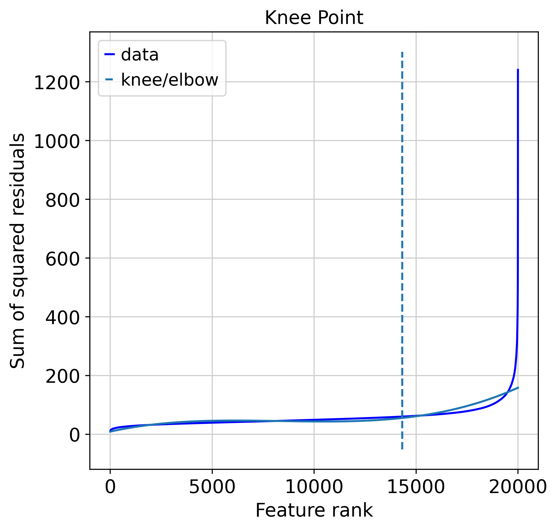
0.9999727878815365
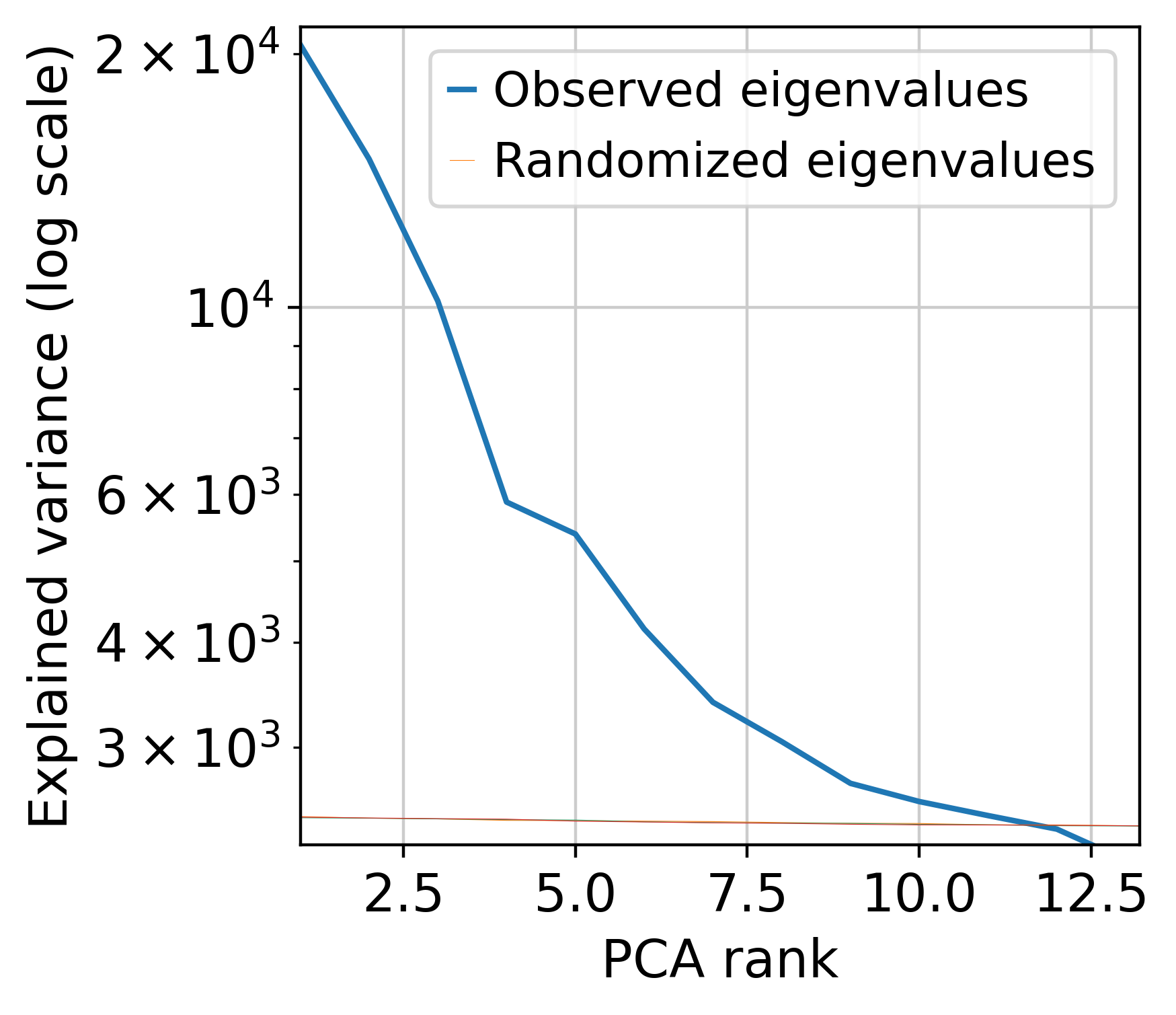
Next, we perform dimensionnality reduction through with PCA and UMAP.
[15]:
muffin.tools.compute_pa_pca(dataset, plot=True)
muffin.tools.compute_umap(dataset)
[15]:
AnnData object with n_obs × n_vars = 52 × 110245
    obs: 'size_factors', 'size_factors_input', 'centered_lfc', 'pi0'
    var: 'Chromosome', 'Start', 'End', 'Strand', 'means', 'variances', 'reg_alpha'
    uns: 'counts_random', 'tot_mapped_counts', 'input_random', 'pca'
    obsm: 'design', 'X_pca', 'X_umap'
    varm: 'PCs'
    layers: 'input', 'normalization_factors', 'residuals'
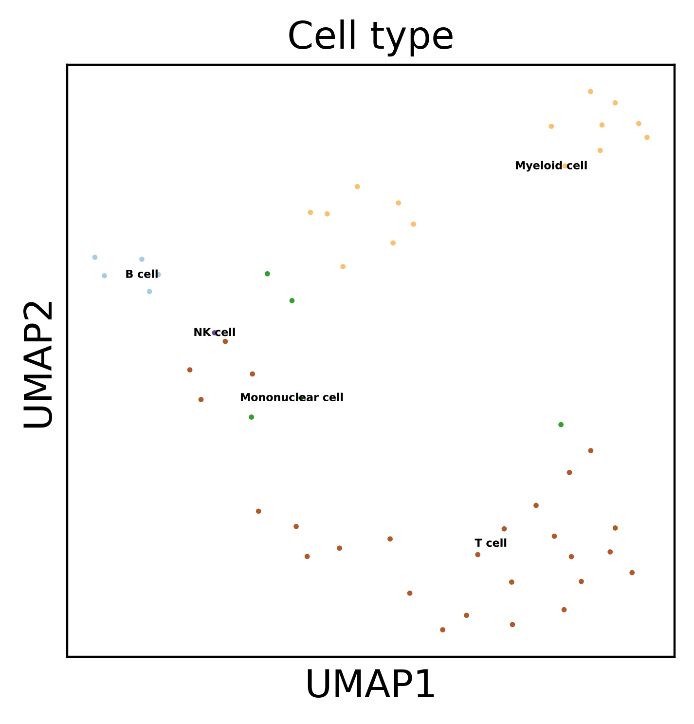
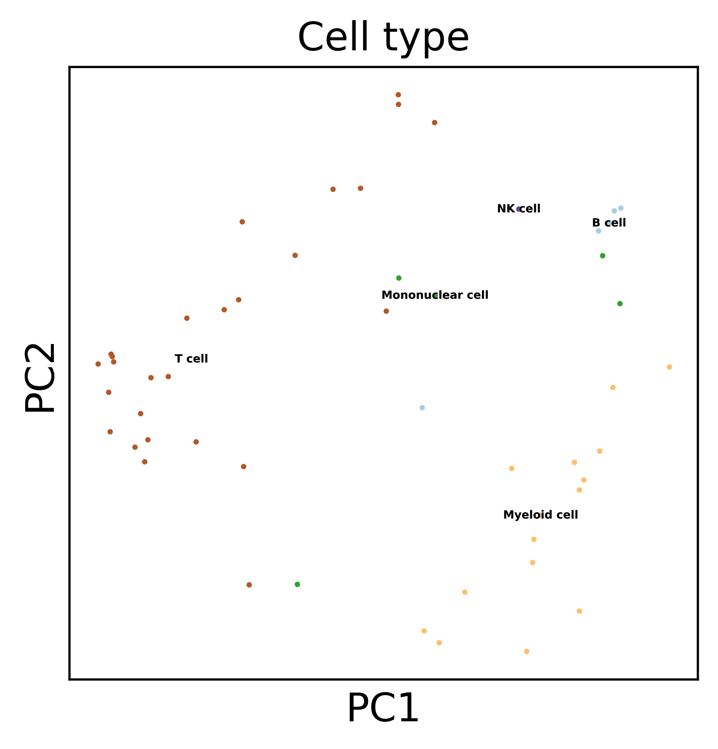
Display the results. Note that we can use scanpy functions here!
[16]:
# Append cell type info to the dataset
dataset.obs["Cell type detailed"] = metadata_chip["Biosample term name"].values
dataset.obs["Cell type"] = metadata_chip["Biosample cell type"].values
sc.pl.umap(dataset, color='Cell type', legend_loc='on data',
                legend_fontsize=4, legend_fontoutline=0.1, s=15.0,
                palette='Paired')
sc.pl.pca(dataset, color='Cell type', legend_loc='on data',
                legend_fontsize=4, legend_fontoutline=0.1, s=15.0,
                palette='Paired')
WARNING: saving figure to file h3k4me3_results/umap.pdf
WARNING: saving figure to file h3k4me3_results/pca.pdf
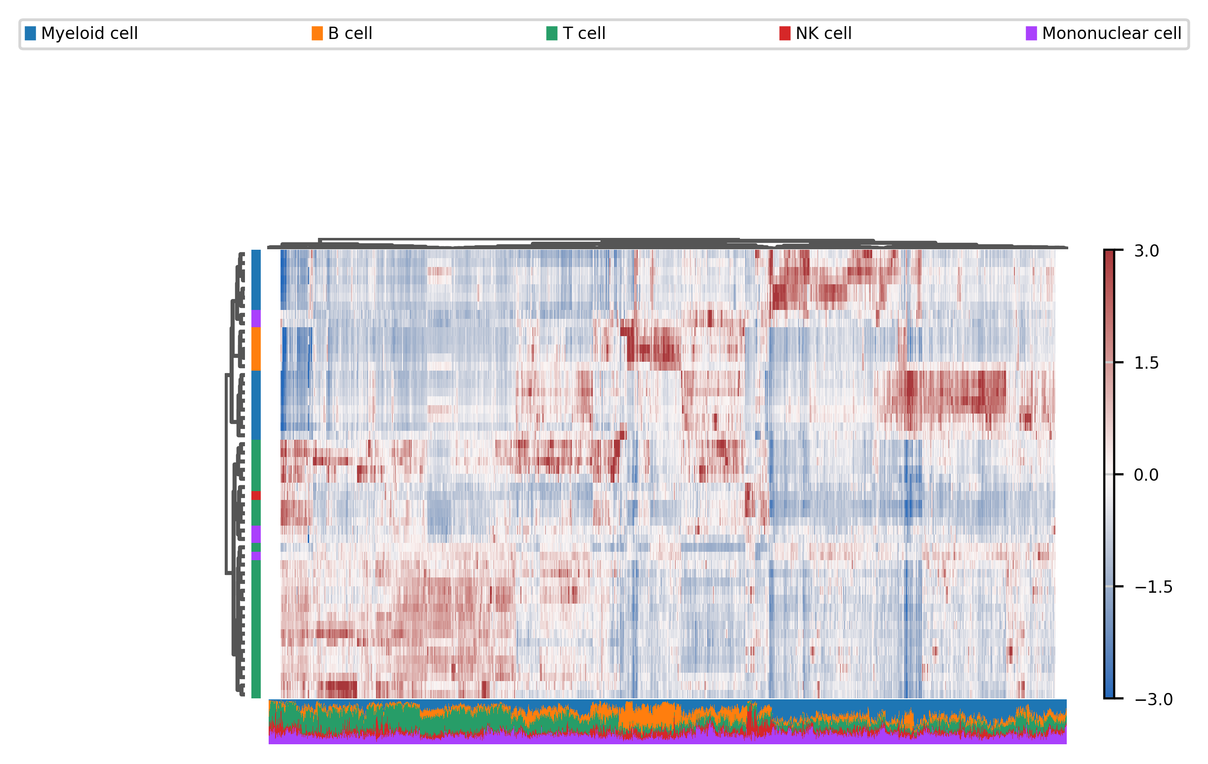
We can also use heatmaps, even if we have a large number of features :
[17]:
print((peaks & hv).sum())
fig, ax = muffin.plots.mega_heatmap(dataset[:, hv&peaks], layer="residuals", label_col="Cell type", vmin=-3, vmax=3)
31290
Let’s find the differentially bound regions between T-cells and B-cells:
[18]:
# First subset our dataset
selected = dataset[(dataset.obs["Cell type"] == "B cell") | (dataset.obs["Cell type"] == "T cell")]
muffin.tools.differential_expression_A_vs_B(selected, category="Cell type",
                                        ref_category="T cell")
Comparing B cell to (reference) T cell
Using DESeq2 with normalization factors per row, per gene
R[write to console]: using pre-existing normalization factors

R[write to console]: estimating dispersions

R[write to console]: gene-wise dispersion estimates

R[write to console]: mean-dispersion relationship

R[write to console]: final dispersion estimates

R[write to console]: fitting model and testing

R[write to console]: -- replacing outliers and refitting for 1157 genes
-- DESeq argument 'minReplicatesForReplace' = 7
-- original counts are preserved in counts(dds)

R[write to console]: estimating dispersions

R[write to console]: fitting model and testing

R[write to console]: using 'apeglm' for LFC shrinkage. If used in published research, please cite:
    Zhu, A., Ibrahim, J.G., Love, M.I. (2018) Heavy-tailed prior distributions for
    sequence count data: removing the noise and preserving large differences.
    Bioinformatics. https://doi.org/10.1093/bioinformatics/bty895
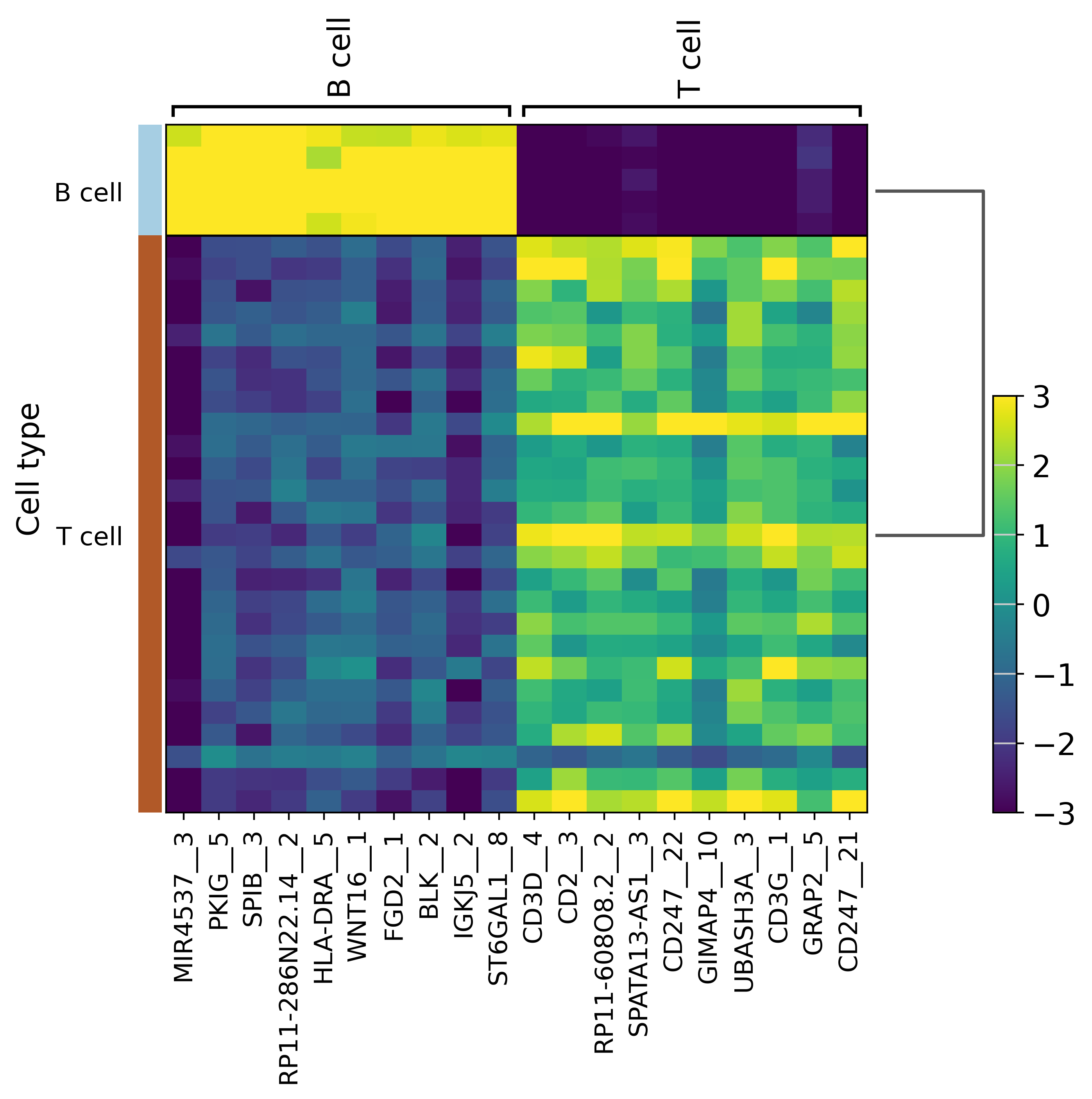
Let’s have a first look at the best markers between B and T cells :
[19]:
sc.pl.rank_genes_groups_heatmap(selected,layer="residuals",
                                use_raw=False, vmin=-3, vmax=3,
                                cmap='viridis')
selected.varm["DE_results"].sort_values("padj")
WARNING: dendrogram data not found (using key=dendrogram_Cell type). Running `sc.tl.dendrogram` with default parameters. For fine tuning it is recommended to run `sc.tl.dendrogram` independently.
WARNING: saving figure to file h3k4me3_results/heatmap.pdf
[19]:
| z-score | log2FoldChange | pvalue | padj | |
|---|---|---|---|---|
| MIR4537__3 | 16.433373 | 5.351551 | 1.103468e-60 | 1.113311e-55 |
| PKIG__5 | 16.050466 | 4.654333 | 5.673613e-58 | 2.862111e-53 |
| SPIB__3 | 15.372901 | 4.865741 | 2.487759e-53 | 8.366498e-49 |
| RP11-286N22.14__2 | 14.659720 | 4.785894 | 1.167530e-48 | 2.944861e-44 |
| HLA-DRA__5 | 14.638806 | 3.962513 | 1.588322e-48 | 3.204979e-44 |
| ... | ... | ... | ... | ... |
| TFEC__1 | -0.631995 | -0.242962 | 5.273903e-01 | 1.000000e+00 |
| IGFBP4__2 | NaN | 1.195152 | NaN | 1.000000e+00 |
| TFEC__4 | 0.763987 | 0.311671 | 4.448748e-01 | 1.000000e+00 |
| RP11-109A6.2__1 | -0.988146 | -0.394602 | 3.230813e-01 | 1.000000e+00 |
| DDX11L1__1 | 0.164114 | 0.114402 | 8.696418e-01 | 1.000000e+00 |
110245 rows × 4 columns
We can already see genes specific to T cells (CD3E, CD3D…) and some specific to B cells (BLNK, BLK…). We can go further and perform a Genomic Regions Enrichment Analysis to get a GSEA of nearby genes.
[20]:
# Retrieve DE regions
DE_indexes = (selected.varm["DE_results"]["padj"] < 0.05) & (np.abs(selected.varm["DE_results"]["log2FoldChange"]) > 1.0)
all_regions = selected.var[["Chromosome", "Start", "End"]]
query = all_regions[DE_indexes]
# Perform GREA
gsea_results = gsea_obj.find_enriched(query, all_regions, cores=16)
gsea_results
[Parallel(n_jobs=16)]: Using backend LokyBackend with 16 concurrent workers.
[Parallel(n_jobs=16)]: Done 2516 tasks      | elapsed:  6.6min
[Parallel(n_jobs=16)]: Done 8216 tasks      | elapsed: 16.7min
[Parallel(n_jobs=16)]: Done 8813 out of 8813 | elapsed: 17.7min finished
[20]:
| P(Beta > 0) | Beta | Total hits | BH corrected p-value | -log10(qval) | -log10(pval) | FC | Name | |
|---|---|---|---|---|---|---|---|---|
| 0 | ||||||||
| GO:0002250 | 6.971654e-48 | 0.562758 | 1963 | 6.144119e-44 | 4.321154e+01 | 4.715666e+01 | 1.755508 | adaptive immune response |
| GO:0046649 | 1.884302e-18 | 0.293050 | 2666 | 8.303178e-15 | 1.408076e+01 | 1.772485e+01 | 1.340509 | lymphocyte activation |
| GO:0042110 | 2.199839e-16 | 0.321682 | 2078 | 5.551631e-13 | 1.225558e+01 | 1.565761e+01 | 1.379447 | T cell activation |
| GO:0045321 | 2.519747e-16 | 0.254236 | 2959 | 5.551631e-13 | 1.225558e+01 | 1.559864e+01 | 1.289475 | leukocyte activation |
| GO:0002684 | 7.413552e-16 | 0.248544 | 2821 | 1.306713e-12 | 1.188382e+01 | 1.512997e+01 | 1.282157 | positive regulation of immune system process |
| ... | ... | ... | ... | ... | ... | ... | ... | ... |
| GO:0051301 | 9.999955e-01 | -0.214479 | 716 | 9.999983e-01 | 7.410858e-07 | 1.961061e-06 | 0.806962 | cell division |
| GO:0019752 | 9.999957e-01 | -0.189734 | 949 | 9.999983e-01 | 7.410858e-07 | 1.886755e-06 | 0.827179 | carboxylic acid metabolic process |
| GO:0043436 | 9.999980e-01 | -0.194738 | 964 | 9.999983e-01 | 7.410858e-07 | 8.733082e-07 | 0.823050 | oxoacid metabolic process |
| GO:0070925 | 9.999982e-01 | -0.189735 | 1025 | 9.999983e-01 | 7.410858e-07 | 7.634767e-07 | 0.827179 | organelle assembly |
| GO:0007017 | 9.999983e-01 | -0.197020 | 907 | 9.999983e-01 | 7.410858e-07 | 7.410858e-07 | 0.821175 | microtubule-based process |
8813 rows × 8 columns
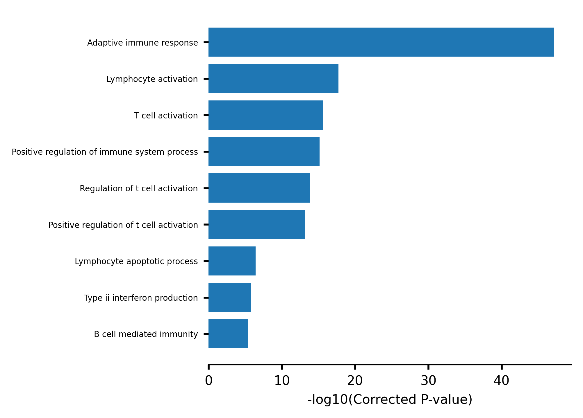
We do observe an enrichment of immune and T/B Cells related terms.
[21]:
import plotly.offline as pyo
pyo.init_notebook_mode()
gsea_clusters = gsea_obj.cluster_treemap(gsea_results, output="h3k4me3_results/cluster_treemap.pdf")
fig, ax = gsea_obj.barplot_enrich(gsea_clusters)
fig.savefig("h3k4me3_results/barplot_enrich.pdf", bbox_inches="tight")
/shared/projects/pol2_chipseq/pkg/miniconda3/envs/muffin_test/lib/python3.10/site-packages/sklearn/metrics/pairwise.py:2182: DataConversionWarning:

Data was converted to boolean for metric yule

/shared/ifbstor1/projects/pol2_chipseq/newPkg/muffin/great.py:605: SettingWithCopyWarning:


A value is trying to be set on a copy of a slice from a DataFrame.
Try using .loc[row_indexer,col_indexer] = value instead

See the caveats in the documentation: https://pandas.pydata.org/pandas-docs/stable/user_guide/indexing.html#returning-a-view-versus-a-copy

/shared/ifbstor1/projects/pol2_chipseq/newPkg/muffin/great.py:608: SettingWithCopyWarning:


A value is trying to be set on a copy of a slice from a DataFrame.
Try using .loc[row_indexer,col_indexer] = value instead

See the caveats in the documentation: https://pandas.pydata.org/pandas-docs/stable/user_guide/indexing.html#returning-a-view-versus-a-copy

/shared/projects/pol2_chipseq/pkg/miniconda3/envs/muffin_test/lib/python3.10/site-packages/kaleido/scopes/base.py:188: DeprecationWarning:

setDaemon() is deprecated, set the daemon attribute instead
We can save our work to avoid recomputing everything. It can easily be re-loaded using : anndata.read_h5ad(path)
[22]:
dataset.write("h3k4me3_results/dataset.h5ad")